Hodge’s Problem

The following theory and problems are adapted from “Theory of Point Estimation” (Lehmann and Casella, 1998) and “Model Selection and the Principle of Minimum Description Length” (Hansen and Yu, 2001).

Consider the following problem by Hodge (Le Cam, 1953). Let $X^n = X_1, \dots, X_n \overset{\text{iid}}{\sim} \mathcal{N}(\theta, 1)$ where $\theta \in \mathbb{R}$ is unknown. We wish to test the hypotheses $H_\theta: \theta = 0$ against $H_1 : \theta \neq 0$, or equivalently choose between the models

\(M_0 = \{\mathcal{N}(0, 1)\} \text{ and } M_1 = \{\mathcal{N}(\theta, 1): \theta \neq 0\}\).

Hodge’s estimator $\hat{\theta}_n$ is defined as \(\hat{\theta}_n = \begin{cases} \bar{X} & \text{if } |\bar{X}| \geq n^{-1/4}\\ 0 & \text{if } |\bar{X}| < n^{-1/4} \end{cases}\)

and thus chooses $M_0$ if and only if $|\bar{X}| < n^{-1/4}$. Notably, the risk $R_n(\theta)$ of this estimator is less than 1 for $\theta$ close to 0 (dependent on $n$) and thus is below the asymptotic variance and Cramer-Rao lower bound making it a superefficient estimator in certain cases.

Alternative, more conventional model selection methods include the Bayesian Information Criterion (BIC), Akaike Information Criterion (AIC), and Minimum Description Length (MDL).

Model Selection

MDL

MDL specifies the complexity of a model in terms of the information theoretic length of a bit string needed to be sent from a sender to a receiver (assuming some common knowlege shared between both parties). From Hansen and Yu (2001), we consider a two-stage coding in which we first quantify the cost $L(\hat{\theta})$ of encoding a parameter and then quantify the cost $L_M(X^n)$ of encoding the data given our model. The cost depends on our level of precision and so the finite parameter space for a given number is discreteized with precision $1 / \sqrt{n}$, reflecting the standard parametric rate of convergence (Hansen and Yu, 2001). We denote the likelihood function of our data given a parameter $\theta$ as $\mathcal{L}_{\theta}$ and our maximum likelihood estimate $\hat{\theta}_n = \bar{X}$.

Thus, we choose $M_0$ iff $MDL_{M_0} < MDL_{M_1}$ which is true, after cancelling terms, when \(|\bar{X}| < (\frac{1}{n}\log n)^{1/2}\).

BIC

BIC is defined as $BIC_M(X^n) = -2\log \mathcal{L}_{\hat{\theta}}(X^n) + k\log n$ and thus here in Hodge’s problem where $k=1$ under $M_1$, BIC is exactly equivalent to MDL up to a scalar multiple and thus the decision rule remains the same.

AIC

AIC is defined as $AIC_M(^n) = -2\log \mathcal{L}_{\hat{\theta}}(X^n) + 2k$. So, in this problem

Thus, we choose $M_0$ iff $AIC_{M_0} < AIC_{M_1}$ which is true, after cancelling terms, when \(|\bar{X}| < (2/n)^{1/2}\).

Model Selection Risks

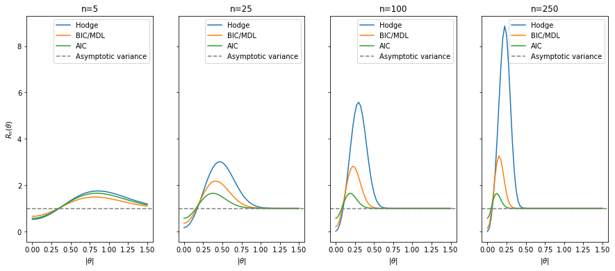
Lehmann and Casella (1998) provide the analytic risk for Hodge’s estimator in Hodge’s problem. Adapting the decision boundary to these alternative model selection scores, we can observe their performance over various sample sizes and $\theta$’s.

import numpy as np
from scipy.stats import norm
from scipy import integrate
import matplotlib.pyplot as plt
%matplotlib inline

def estimator_risk(theta, n, a=0, threshold=lambda n: n**(-1/4)):
    """
    Analytical risk for Hodges example
    Source: Theory of Point Estimation (pg 442, Lehmann and Casella, 1998)
    
    Parameters
    ----------
    theta : mean of the normal distribution
    n : number of samples observed
    a : coefficient of estimate under the threshold
    threshold : value at which the model changes, default Hodge's
    
    Notes
    -----
    Estimator \delta_n = \bar{X} if |\bar{X}| \geq threshold else a\bar{X}    
    
    Risk R_n(\theta) = nE[(\delta_n - \theta)^2]
    
    Hodge's estimator threshold = n^{-1/4}
    """
    n_2 = n ** (1/2) 
    z = threshold(n) * n_2

    I_ceil = z - n_2 * theta
    I_floor = -z - n_2 * theta
    integral = integrate.quad(lambda x: x**2 * norm.pdf(x), I_floor, I_ceil)[0]

    R_n = 1 - (1 - a ** 2) * integral
    R_n += n * theta ** 2 * (1 - a) ** 2 * (norm.cdf(I_ceil) - norm.cdf(I_floor))
    R_n += 2 * n_2 * theta * a * (1 - a) * (norm.pdf(I_ceil) - norm.pdf(I_floor))

    return R_n

hodges_thresh = lambda n: n ** (-1/4)
bic_thresh = lambda n: (np.log(n) / n) ** (1/2)
aic_thresh = lambda n: (2 / n) ** (1/2)

theta_range = np.linspace(0, 1.5, 61)
n_range = [5, 25, 100, 250]

fig, axes = plt.subplots(1, 4, figsize=(15, 6), sharex=True, sharey=True)
model_names = ['Hodge', 'BIC/MDL', 'AIC']
models = [hodges_thresh, bic_thresh, aic_thresh]
for n, ax in zip(n_range, axes):
    for name, model in zip(model_names, models):
        risk = [estimator_risk(theta, n, a=0, threshold=model) for theta in theta_range]
        ax.plot(theta_range, risk, label=f'{name}')

    ax.axhline(1, c='grey', ls='--', label='Asymptotic variance')
    ax.set_xlabel(r'$|\theta|$')
    ax.set_xticks(np.linspace(0, 1.5, 7))
    ax.legend()
    ax.set_title(f'n={n}')
    
axes[0].set_ylabel(r'$R_n(\theta)$')
plt.show()    

hodges_thresh = lambda n: n ** (-1/4)
bic_thresh = lambda n: (np.log(n) / n) ** (1/2)
aic_thresh = lambda n: (2 / n) ** (1/2)

theta_range = np.linspace(0, 1.5, 61)
n_range = [5, 25, 100, 250]

fig, axes = plt.subplots(1, 3, figsize=(15, 6), sharex=True, sharey=True)
model_names = ['Hodge', 'BIC/MDL', 'AIC']
models = [hodges_thresh, bic_thresh, aic_thresh]
for i, (name, model) in enumerate(zip(model_names, models)):
    ax = axes[i]
    risks = [
        [estimator_risk(theta, n, a=0, threshold=model) for theta in theta_range]
        for n in n_range
    ]
    
    for n, risk in zip(n_range, risks):
        ax.plot(theta_range, risk, label=f'n={n}')
    ax.axhline(1, c='grey', ls='--', label='Asymptotic variance')
    ax.set_xlabel(r'$|\theta|$')
    ax.set_xticks(np.linspace(0, 1.5, 7))
    ax.legend()
    ax.set_title(name)
    
axes[0].set_ylabel(r'$R_n(\theta)$')
plt.show()    

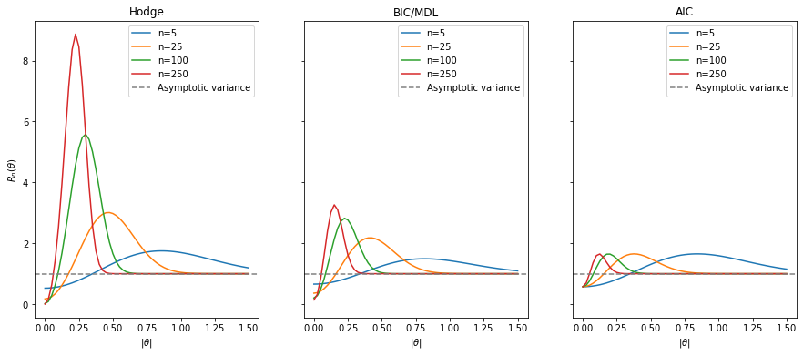
Notably, all estimators are superefficient for small $\theta$, requiring smaller $\theta$ the larger $n$ is. AIC, however, appears to maintain almost constant risk even as sample size grows whereas BIC (equivalently MDL) and even moreso Hodge’s estimator have larger risks that grow as $n$ increases on a vanishingly small set of possible $\theta \in \mathbb{R}$.