My 2020 Strava running year in review

9 minute read

Published: December 31, 2020

My 2020 Strava running year in review

At the end of May, I started training for the Baltimore Marathon in October and also acquired a Garmin GPS watch to upload my training logs to Strava. Unfortunately, the marathon became virtual and I ran into some Achilles tendon issues in September. That being said, I got into the best shape of my life so far and had a lot of fun. But having all the data on Strava allowed me to dig into it a bit more, after they emailed me my account data, including a csv file of all my activities (and a pdf telling me what companies they were sending my data too, expected but still slightly unnerving).

So here is my 2020 running year in review!

import numpy as np
import pandas as pd
import matplotlib.pyplot as plt
%matplotlib inline
import seaborn as sns
sns.set(style="darkgrid")

First we need to load the data, and make some nice variables for to work with

activities = pd.read_csv('./activities.csv')
# Only runs
activities = activities[activities['Activity Type'] == 'Run']
# km -> miles
activities['Distance'] = (activities['Distance'] / 1.609).round(2)
activities['Grade Adjusted Distance'] = (activities['Distance'] / 1.609).round(2)
activities['Elevation Gain'] = (activities['Elevation Gain'] / 1000 / 1.609).round(2)
activities['Elevation Loss'] = (activities['Elevation Gain'] / 1000 / 1.609).round(2)
# sec -> min
activities[['Elapsed Time', 'Moving Time']] = (activities[['Elapsed Time', 'Moving Time']] / 60).round(2)
# time and distance
activities[['Max Speed', 'Average Speed']] = (activities[['Max Speed', 'Average Speed']] / 1.609 * 60).round(2)
# Format dates
activities['Activity Date'] = pd.to_datetime(activities['Activity Date'], format='%b %d, %Y, %H:%M:%S %p')
activities['Day of week'] = activities['Activity Date'].dt.day_name()
activities['Day'] = activities['Activity Date'].dt.strftime("%b %d, %Y")
# Other features of interest
activities['Minutes per mile'] = activities['Moving Time'] / activities['Distance']

Here’s what some of the entries look like.

activities.head(2)

	Activity ID	Activity Date	Activity Name	Activity Type	Activity Description	Elapsed Time	Distance	Relative Effort	Commute	Activity Gear	...	Weather Visibility	UV Index	Weather Ozone	translation missing: en-US.lib.export.portability_exporter.activities.horton_values.jump_count	translation missing: en-US.lib.export.portability_exporter.activities.horton_values.total_grit	translation missing: en-US.lib.export.portability_exporter.activities.horton_values.avg_flow	translation missing: en-US.lib.export.portability_exporter.activities.horton_values.flagged	Day of week	Day	Minutes per mile
0	3444448060	2020-05-13 12:41:35	Morning Run	Run	NaN	31.87	4.31	8.0	False	NaN	...	NaN	NaN	NaN	NaN	NaN	NaN	NaN	Wednesday	May 13, 2020	7.366589
1	3449767282	2020-05-14 01:17:08	Morning Run	Run	Felt great starting out. Hills hurt. Maybe wen...	49.33	6.83	73.0	False	NaN	...	NaN	NaN	NaN	NaN	NaN	NaN	NaN	Thursday	May 14, 2020	7.125915

2 rows × 81 columns

Let’s check out my speed over time. It looks like there are some outliers, I can definiely recall some funky things my watch did.

sns.lineplot(data=activities, x='Activity Date', y='Minutes per mile', marker='o')
plt.show()

png

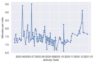
We can look at the slowest runs and fastest runs I had. There are some entries that look like they are the results of errors, so we can go ahead and remove them.

activities.sort_values(by = 'Minutes per mile').head(5)[['Activity Description', 'Minutes per mile', 'Day of week']]

	Activity Description	Minutes per mile	Day of week
93	This is what happens when a Baltimore marathon...	6.612903	Wednesday
77	First shirted run in a while, 55 deg out of no...	6.690227	Tuesday
83	4x1600m (5:36, 5:34, 5:33, 5:30). Tendon didn'...	6.695608	Tuesday
60	1200 pacing for Tommy's 5k	6.723404	Saturday
82	Am now of the gloves > long sleeves opinion. W...	6.800705	Sunday

activities.sort_values(by = 'Minutes per mile',).tail(5)[['Activity Description', 'Minutes per mile']]

	Activity Description	Minutes per mile
94	Recovery back. Is my other Achilles screwed? T...	8.246753
113	Nice and chill, getting longer	8.347887
114	Some intermittent running with Adam	9.101796
11	Reunion with the boys. Shin splints, not sure ...	9.397138
25	No, I didn't run through the middle of the lak...	9.506643

activities = activities.drop(index=[25])

For fun we can start with some summary statistics.

total_runs = len(activities)
print(f'You ran {total_runs} total runs this year!')
total_miles = sum(activities['Distance'])
print(f'That\'s {int(total_miles)} miles (wow).')
total_minutes = sum(activities['Moving Time'])
total_hours = total_minutes / 60
print(f'That\'s {int(total_minutes)} minutes ({int(total_hours)} hours!).')
total_calories = sum(activities['Calories'].dropna())
total_burgers = total_calories / 354
print(f'Strava says {int(total_calories)} calories burned (That\'s {int(total_burgers)} burgers).')
total_elevation = sum(activities['Elevation Gain'])
print(f'And {int(total_elevation)} miles climbed (Baltimore is pretty flat)')

You ran 116 total runs this year!
That's 889 miles (wow).
That's 6585 minutes (109 hours!).
Strava says 94221 calories burned (That's 266 burgers).
And 11 miles climbed (Baltimore is pretty flat)

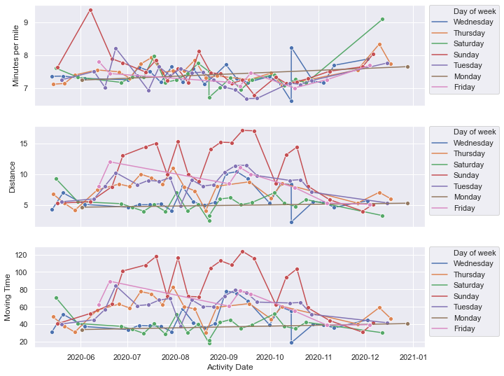
Now we can go ahead and see what my performance and training looked like across each day of the week. My training schedule was pretty consistent as to what types of runs were done on which days and that’s reflected in these plots. We clearly see the buildup and then decrease after I injured my Achilles tendon in late September.

cols = ['Minutes per mile', 'Distance', 'Moving Time']
f, axs = plt.subplots(len(cols), 1, figsize=(10, len(cols)*3), sharex=True)
for i, c in enumerate(cols):
    df = activities[['Activity Date', 'Day of week', c]]
    # df[c] = df[c].rolling(7).mean()
    sns.lineplot(data=df, x='Activity Date', y=c, hue='Day of week', marker='o', ax=axs[i])
    axs[i].legend(bbox_to_anchor=(1.01, 1), loc=2, borderaxespad=0.)
plt.show()

png

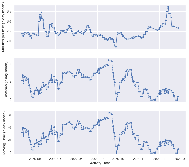
The daily information is a bit noisy, so we can also look at the same data as a weekly (7 day) moving average. Some of the trends a more noticeable and some sharp changes in my training due to work or injury become more apparent.

df = activities[
    ['Distance', 'Moving Time', 'Activity Date', 'Activity Description']
].resample('D', on='Activity Date').sum().reset_index()
df['Minutes per mile'] = df['Moving Time'] / df['Distance']
df['Activity Date'] = pd.to_datetime(df['Activity Date'])
df['Day of week'] = df['Activity Date'].dt.day_name()

cols = ['Minutes per mile', 'Distance', 'Moving Time']
f, axs = plt.subplots(len(cols), 1, figsize=(10, len(cols)*3), sharex=True)
for i, c in enumerate(cols):
    df[f'{c} (7 day mean)'] = df[c].rolling(7, min_periods=1).mean()
    sns.lineplot(data=df, x='Activity Date', y=f'{c} (7 day mean)', marker='o', ax=axs[i])
plt.show()

png

In the interest of my performance prior to injury, we can identify the exact day with the help of my logged description. We can go ahead and look at my performance up to this point, where my training became a bit rocky as I recovered.

activities[activities['Activity Description'].str.contains('tendon|achilles', na=False, case=False)].head(1)

	Activity ID	Activity Date	Activity Name	Activity Type	Activity Description	Elapsed Time	Distance	Relative Effort	Commute	Activity Gear	...	Weather Visibility	UV Index	Weather Ozone	translation missing: en-US.lib.export.portability_exporter.activities.horton_values.jump_count	translation missing: en-US.lib.export.portability_exporter.activities.horton_values.total_grit	translation missing: en-US.lib.export.portability_exporter.activities.horton_values.avg_flow	translation missing: en-US.lib.export.portability_exporter.activities.horton_values.flagged	Day of week	Day	Minutes per mile
83	4096403891	2020-09-22 10:57:43	Morning Run	Run	4x1600m (5:36, 5:34, 5:33, 5:30). Tendon didn'...	87.62	9.79	59.0	False	NaN	...	NaN	NaN	NaN	NaN	NaN	NaN	NaN	Tuesday	Sep 22, 2020	6.695608

1 rows × 81 columns

activities[activities['Activity Description'].str.contains('tendon|achilles', na=False, case=False)].head(1).iloc[0,4]

"4x1600m (5:36, 5:34, 5:33, 5:30). Tendon didn't feel great on the way back so might have to take some days off."

training_df = df.iloc[:df[df['Activity Date'] == '2020-09-22'].index[0]+1]
training_df = training_df.assign(Day=training_df.index)

import statsmodels.api as sm
endog = training_df.dropna()['Minutes per mile (7 day mean)']
exog = sm.add_constant(training_df.dropna()['Day'])
ols = sm.OLS(endog, exog)
results = ols.fit()

c = 'Minutes per mile'
f, ax = plt.subplots(1, 1, figsize=(10, 3))
ax.plot(
    training_df.dropna()['Activity Date'],
    results.fittedvalues, 'r--.', label=f"y={results.params.Day:.4f}x + {results.params.const:.2f}")
sns.lineplot(
    data=training_df,
    x='Activity Date', y=f'{c} (7 day mean)', marker='o', ax=ax, label='Rolling mean')
plt.xticks(rotation=30, ha='right')
plt.title('Average time per mile during marathon training period', fontsize=15)
plt.show()
min_per_mile_change = results.params.Day * training_df.Day.iloc[-1]
print(f'Average minutes per mile decreased by {-min_per_mile_change*60:.1f} seconds over the course of the training')

png

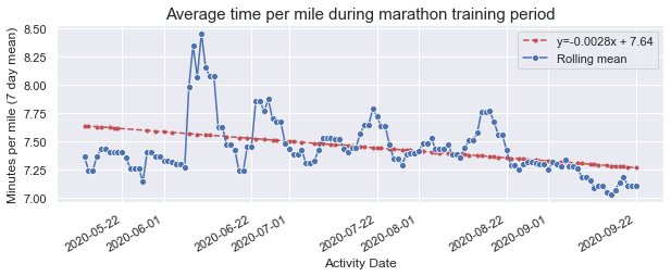
Average minutes per mile decreased by 22.2 seconds over the course of the training

I’ve gone ahead and fit a linear regression to the 7 day moving average which is a problematic thing to do but nonetheless quantifies the trend downward we can see visually. My training towards the end got pretty consistent with the help of a friend although the increase we see in mid-August was the result of being super busy with Fellowship applications and not having as much time to train.

cols = [
    'Elapsed Time', 'Moving Time', 'Minutes per mile', 'Distance', 'Grade Adjusted Distance',
    'Elevation Gain', 'Relative Effort', 'Max Speed', 'Average Speed', 'Average Cadence',
    'Max Heart Rate', 'Average Heart Rate', 'Calories'
]
df = activities[cols]

# Compute the correlation matrix
corr = df.corr()
mask = np.triu(np.ones_like(corr, dtype=bool))

sns.set_style("white")
f, ax = plt.subplots(figsize=(11, 9))
# Draw the heatmap with the mask and correct aspect ratio
heatmap = sns.heatmap(corr, mask=mask, center=0, cmap='RdBu_r',
            square=True, linewidths=.5, cbar_kws={"shrink": 0.75})
plt.xticks(rotation=45, ha='right')
plt.title('Correlations over logged activities', fontsize=15)
plt.show()

png

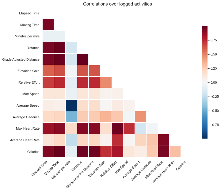
Not too many surprises at the relationships between some of this data. A lot of things are heavily correlated that would be expected, i.e. Distance and Relative Effort. Average heart rate is actually not that strongly correlated with many of the variables, excet for relative effort which may be a sign as to how that’s computed.

Minutes per mile, what one will see listed on every run, is strongly negatively correlated with the average speed which is a good sanity check as they are inverses of one another. We also see a negative correlation with average cadence, which means when I run faster I’m getting in more steps per distance which also makes sense.

Interestingly, however, we see a slight negative correlaton, at least not positive, between minutes per mile and distance! This confirms to me that I actually tend to speed up on some of my longer runs. I know I’m not the only runner to do that.

sns.set_style("darkgrid")
f, ax = plt.subplots(figsize=(11, 6))
sns.swarmplot(data=activities, x='Day of week', y='Distance', palette="Set3", linewidth=1)
sns.despine(left=True, bottom=True)
plt.show()

png

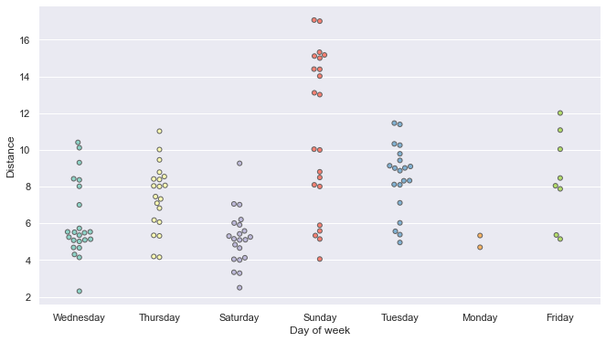
And here is a big surprise. From the end of May through the end of December, I only ever ran on a Monday twice! My training schedule always had long runs on Sunday and a rest day on Monday, so this shouldn’t be too unexpected but still comes as a surprise.

Ronan Perry

My 2020 Strava running year in review